Introduction

Night Lights data (Yi et al., 2014) has been able to determine urbanization processes, and so far, we have witness expansion sets of analysis. Its’ ability to track urban sprawl expansion, the urban environment, and its’ level of activity are highly suitable. While it may detect urban expansion, the project will query its’ ability to query the contrary.

In context, the Defense Meteorological Satellite Program is a widely quoted data. It is a collection of two satellites that are solar coordinated, which one satellite is in a dawn - dusk orbit, and the second in a day - night orbit. The DMSP Operational Linescan System (OLS) data sets are utilized for this project. As stated on NOAA’s page,

“The wide swath widths provide for global coverage four times a day: dawn, day, dusk, night.”

“With sunlight eliminated, the light intensification makes it possible to detect city lights, gas flares, and fires.”

As such, the project deem its’ specific capabilities for detection for statistical data collection fit for the usage of consideration.

In reproducing the widely cited data in a standardized manner, relevant data sets were tracked down according to the inheritance after intragovernmental agencies merger. The NOAA’s National Centers for Environmental Information (NCEI) supports DoD’s data archival for the DMSP sensors, which the U.S. Air Force Global Weather Central sends DMSP data to NCEI. Archival operation was established in March of 1992, and began receiving data on a daily basis in September of 1992. The mentioned time series and grandfathered collaboration across government agencies will be used for streamlining reproducible of the research, but in a compression manner.

Crucially, a city’s existence relies on its’ inhabitants, and tracking of its activity can be intermediate through lights. The population’s activity of light usage measurement a good way to detect its’ vibrancy or inactivity. Many publications have the manner of understanding it through growth phases, but the project will attempt to achieve proof on concept in a contracting manner rather than expansion, in even timed series for more contrasting effects. Therefore, the Rust Belt cities offer intriguing insights of shrinking cities and its population.

Methodology: Visualization of the Cities

As for tidying the data set, the project will utilize the libraries as commented in the codes. The loop function works by utilizing “foreach library. It will run the cities that were selected above.The visualization process will use a loop function for both years to geocode and will be assigned with relevant variables. Namely the process order is as follow:

Firstly in the loop function, the cities will be geocoded and assigned temporarily before merged.

Secondly, the bounding box will be established before being merged with the satellite image.

Thirdly, the referenced codes (Chen, 2017) will visually inspect rasters by color coding raster values on a map using k-means clustering algorithm.

Lastly, the sampled radiance level will be plotted to reveal visually of the night lights in relevant cities.

The geocoded cities coordinates are also saved to prevent frequent queries through the ggpmap library as Google’s Term of Policies limits queries. As for the files displayed, they are PNG files generated from cropping the bounding box parameters with the nightlights dotted according to spatial projection referenced.

As for faster website loading, the visualization loads the PNG files generated rather than running the processing of visualization that is computational intensive.

#Visualizing Cities for Year 2014
########################################################################################
coords2014=data.frame()

##Loop
for(i in 1:length(cities)){
  
  ##Coords
  temp_coord=geocode(override_limit = TRUE, cities[i], source = c("google", "dsk"), key = "AIzaSyBlAs3JB7y49JPpUWMQvZGdie2ZqWNmZss")
  coords2014=rbind(coords2014,temp_coord)
  
  #Bounding Box
  boundbox=extent(temp_coord$lon - 1, temp_coord$lon + 1,
                  temp_coord$lat - 0.25, temp_coord$lat + 0.25)
  
  #Pasting Boundbox to Raster
  rc=crop(rast2014, boundbox)    
  
  ##Rescale brackets
  sampled=as.vector(rc)
  clusters=15
  clust=kmeans(sampled,clusters)$cluster
  combined=as.data.frame(cbind(sampled,clust))
  brk=sort(aggregate(combined[,1], list(combined[,2]), max)[,2])
  
  #Plots
  plot(rc, breaks=brk, col=colorRampPalette(c("#001a4d","#0066FF", "yellow"))(clusters), 
       legend=F,yaxt='n',xaxt='n',frame = F, asp=1.5)
  text(temp_coord$lon ,temp_coord$lat + 0.15,
       substr(cities[i],1,regexpr(",",cities[i])-1), 
       col="white", cex=1.25)
  
  rm(combined)
}

#Saving Geocodes
write.csv(coords2014,file ="data/coords2014.csv" )
###############################################################################################

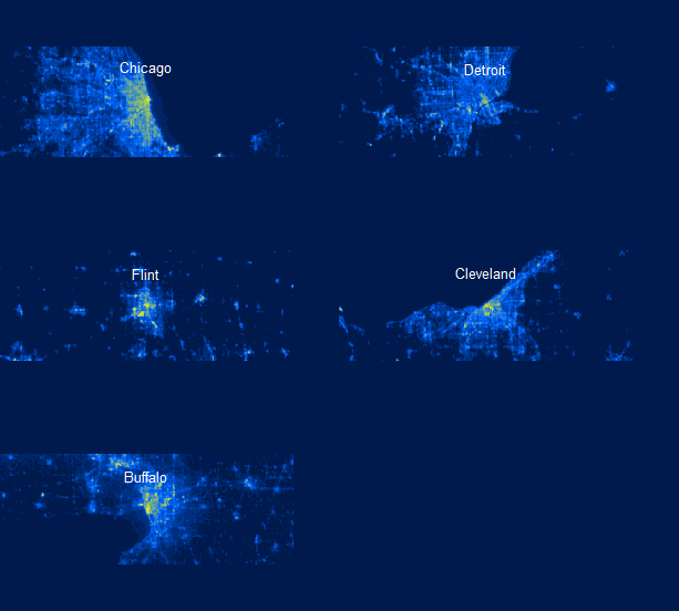
2014

#Visualizing Cities for Year 2016
coords2016=data.frame()

##Loop
for(i in 1:length(cities)){
  
  ##Coords
  temp_coord=geocode(override_limit = TRUE, cities[i], source = c("google", "dsk"), key = "AIzaSyBRzBKmnnK9vwKDrqSBR6olexFThQNWU-8")
  coords2016=rbind(coords2016,temp_coord)
  
  #Bounding Box
  boundbox=extent(temp_coord$lon - 1, temp_coord$lon + 1,
              temp_coord$lat - 0.25, temp_coord$lat + 0.25)
  
  #Pasting Boundbox to Raster
  rc=crop(rast2016, boundbox)    
  
  ##Rescale brackets
  sampled=as.vector(rc)
  clusters=15
  clust=kmeans(sampled,clusters)$cluster
  combined=as.data.frame(cbind(sampled,clust))
  brk=sort(aggregate(combined[,1], list(combined[,2]), max)[,2])
  
  #Plots
  plot(rc, breaks=brk, col=colorRampPalette(c("#001a4d","#0066FF", "yellow"))(clusters), 
       legend=F,yaxt='n',xaxt='n',frame = F, asp=1.5)
  text(temp_coord$lon ,temp_coord$lat + 0.15,
       substr(cities[i],1,regexpr(",",cities[i])-1), 
       col="white", cex=1.25)
  
  rm(combined)
}

#Saving Geocodes  
write.csv(coords2016,file ="data/coords2016.csv" )
#########################################################################################

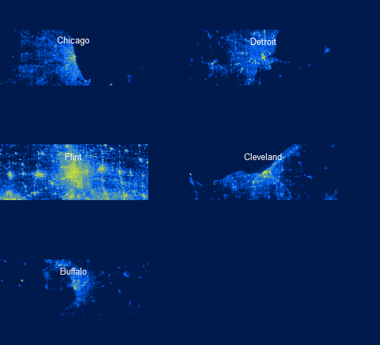
2016

Methodology: Histogram of Satellite Image (Raster Data to Vector Data Conversion)

The codes below referenced (Chen, 2017) from the guidelines given by Department of Commerce will convert GeoTIFFs to vector data. Again, it will use a loop for both years.

##Histogram 2016
histogram=function(shp,rast2016,i){
  
  #Extract one polygon based on index value i
  polygon=shp[i,] #extract one polygon
  extent=extent(polygon) #extract the polygon extent 
  
  #Raster extract
  outer=crop(rast2016, extent) #extract raster by polygon extent
  inner=mask(outer,polygon) #keeps values from raster extract that are within polygon
  
  #Convert cropped raster into a vector
  #Specify coordinates
  coords2016=expand.grid(seq(extent@xmin,extent@xmax,(extent@xmax-extent@xmin)/(ncol(inner)-1)),
                        seq(extent@ymin,extent@ymax,(extent@ymax-extent@ymin)/(nrow(inner)-1)))
  
  #Convert raster into vector
  data=as.vector(inner)
  
  #tidying data into dataframe
  data=cbind(as.character(shp@data$CBSAFP[i]),coords2016, data) 
  colnames(data)=c("GEOID","lon","lat","avg_rad") #note that 
  data=data[!is.na(data$avg_rad),] #keep non-NA values only
  
  return(data)
}

##Histogram 2014
histogram=function(shp,rast2014,i){
  
  #Extract one polygon based on index value i
  polygon=shp[i,] #extract one polygon
  extent=extent(polygon) #extract the polygon extent 
  
  #Raster extract
  outer=crop(rast2014, extent) #extract raster by polygon extent
  inner=mask(outer,polygon) #keeps values from raster extract that are within polygon
  
  #Convert cropped raster into a vector
  #Specify coordinates
  coords2014=expand.grid(seq(extent@xmin,extent@xmax,(extent@xmax-extent@xmin)/(ncol(inner)-1)),
                         seq(extent@ymin,extent@ymax,(extent@ymax-extent@ymin)/(nrow(inner)-1)))
  #Convert raster into vector
  data=as.vector(inner)
  
  #package data in neat dataframe
  data=cbind(as.character(shp@data$CBSAFP[i]),coords2014, data) 
  colnames(data)=c("GEOID","lon","lat","avg_rad") #note that 
  data=data[!is.na(data$avg_rad),] #keep non-NA values only
  
  return(data)
}

Methodology: Extracting CBSA Geocoded Areas for Population and Totalling Night Lights from Radiance Data

In order to obtain the necessary radiance statistics within the geographic boundaries specified, the five cities, the project will utilize two cores (process intensive), limited by resource capacity, to speed up the extraction process.

Once the extraction is done, it will have the sum of the total night lights with the relevant “GEOID”, in this case, the CBSA areas selected. Then, the process of merging it with the Metropolitan Statistical Area’s population statistic can be done.

The process described is performed for both years recursively to obtain the necessary statistics for plotting.

#Plotting
#Scatterplot with Trendline of "TNL and Population"

##Year 2016
registerDoParallel(cores=2)
extract2016=foreach(i=1:nrow(msa2016@data), .combine=rbind, .packages="raster") %dopar% {
  data=histogram(msa2016,rast2016,i)
  data.frame(GEOID = data$GEOID[1],sum = sum(data$avg_rad))
}
extract2016$GEOID=as.numeric(as.character(extract2016$GEOID))

##Merge data
merge2016=merge(extract2016, msa_pop2016[,c("CBSA","NAME","POPESTIMATE2016")],by.x="GEOID",by.y="CBSA")

colnames(merge2016)=c("GEOID","TNL","MSA","Population")

#Saving Large Extracted Data 2016
write.csv(extract2016,file ="data/extract2016.csv" )

    

##Year 2014
registerDoParallel(cores=2)
extract2014=foreach(i=1:nrow(msa2014@data), .combine=rbind, .packages="raster") %dopar% {
  data=histogram(msa2014,rast2014,i)
  data.frame(GEOID = data$GEOID[1],sum = sum(data$avg_rad))
}
extract2014$GEOID=as.numeric(as.character(extract2014$GEOID))

#Saving Large Extracted Data 2014  
write.csv(extract2014,file ="data/extract2014.csv" )

##Merge data
merge2014=merge(extract2014, msa_pop2014[,c("CBSA","NAME","POPESTIMATE2014")],by.x="GEOID",by.y="CBSA")

colnames(merge2014)=c("GEOID","TNL","MSA","Population")

Results

Plots ,which are scatterplots, are done logarithmically due to large sum size and magnitude for Total Night Lights (TNL) against Population.

#Scatterplot with Trendline of "TNL and Population"
#Plotting for year 2014 
ggplot(merge2014, aes(log(TNL), log(Population))) +
  geom_hex() +
  geom_smooth(aes(color = log(TNL))) +
  labs(title="Total Night Time Light vs Population 2014")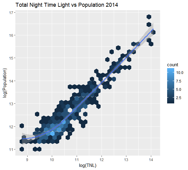

2014

#Plotting for year 2016
ggplot(merge2016, aes(log(TNL), log(Population))) +
  geom_hex() +
  geom_smooth(aes(color = log(TNL))) +
  labs(title="Total Night Time Light vs Population 2016")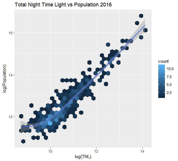

2016

Conclusions

Total night lights in summation is a good proxy for estimating population. It is possible to merge geographically relevant areas quickly with satellite images accurately. However, the process is computationally intensive, but significant. As for achieving the objective of the project, it has proven itself as a concept. The merger of the satellite image’s radiance with geocoded base maps allows quick mapping of the selected cities with their radiance level in an overall manner for comparison across time in montages.

The plotted chart clearly shows a good fit of using the sum of night lights data by DMSP OLS in relation to the population estimates by US Census Bureau, even on shrinking cities. The plot comparison between the two years show the trend line being sticky despite the drop in sum of night lights as the years goes by.

Future studies with more time intervals and shorter time intervals would yield better detailed visualization and more insights. Provided that there is better resources for computing capacity, dynamic visualization would be inspirational for better scale and precision.

References

Yi, K., Tani, H., Li, Q., Zhang, J., Guo, M., Bao, Y., Wang, X. and Li, J. (2014). Mapping and Evaluating the Urbanization Process in Northeast China Using DMSP/OLS Nighttime Light Data. Sensors, 14(2), pp.3207-3226.

Ngdc.noaa.gov. (2017). NOAA/NGDC - Earth Observation Group - Defense Meteorological Satellite Program, Boulder. [online] Available at: https://www.ngdc.noaa.gov/eog/viirs/download_dnb_composites.html .

Huang, B. 2017, Comprehensive Geographic Information Systems, Elsevier, US.

Chen, J. (2017). CommerceDataService/tutorial_viirs_part1. [online] GitHub. Available at: https://github.com/CommerceDataService/tutorial_viirs_part1 .